
Regularization in Machine learning (Ridge and Lasso)
Introduction to Regularization
Regularization is a crucial technique in machine learning used to prevent overfitting, which occurs when a model learns the training data too well, including its noise and outliers. An overfit model performs excellently on training data but poorly on unseen test data.
Why Do We Need Regularization?
When we train machine learning models, especially complex ones with many parameters, they tend to fit the training data perfectly. However, this can lead to the model learning the noise in the data rather than the underlying pattern. Regularization helps by:
- Reducing model complexity
- Preventing overfitting
- Improving generalization to new, unseen data
- Handling multicollinearity in regression problems
How Regularization Works
Regularization works by adding a penalty term to the loss function that the model tries to minimize during training. This penalty term is proportional to the magnitude of the model parameters (weights). By penalizing large weights, regularization encourages the model to use smaller weights, leading to a simpler model that is less likely to overfit.
The general form of a regularized loss function is:
Regularized Loss = Original Loss + λ * Regularization Term
Where:
- Original Loss is the standard loss function (e.g., mean squared error for regression)
- λ (lambda) is the regularization strength (hyperparameter)
- Regularization Term is the penalty based on the model’s weights
Types of Regularization
There are several types of regularization techniques, but two of the most common ones in linear and logistic regression are:
- Ridge Regression (L2 Regularization)
- Lasso Regression (L1 Regularization)
Let’s explore each of these in detail.
Ridge Regression (L2 Regularization)
Ridge regression adds a penalty term that is proportional to the square of the magnitude of the coefficients.
Mathematical Formulation
For linear regression, the standard cost function is:
J(θ) = MSE(θ) = (1/n) * Σ(y_i - ŷ_i)²
Ridge regression adds the L2 norm of the parameter vector:
J(θ) = MSE(θ) + λ * Σ(θ_j)²
Where:
- MSE(θ) is the mean squared error
- λ is the regularization strength
- θ_j are the model parameters (excluding the bias term θ_0)
Key Characteristics of Ridge Regression
- Shrinkage: Ridge regression shrinks the coefficients towards zero, but never exactly to zero.
- Feature Selection: It doesn’t perform feature selection as it keeps all the features in the model.
- Multicollinearity: Excellent for handling multicollinearity (high correlation between features).
- Analytical Solution: Has a closed-form solution.
- Effect on Bias-Variance: Reduces variance but increases bias.
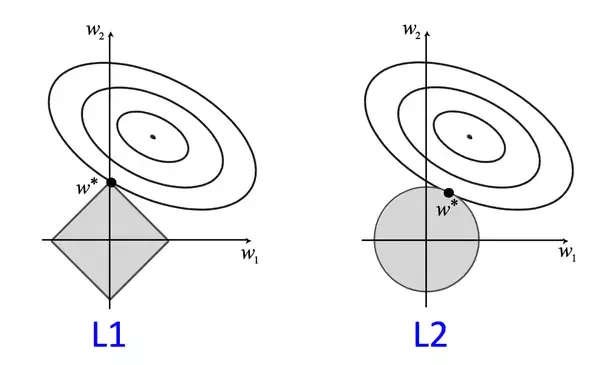
Visual Representation
In ridge regression, the penalty term creates a constraint that can be visualized as a circle in parameter space. The optimization process finds the point where this circle intersects with the contour lines of the loss function.
Lasso Regression (L1 Regularization)
Lasso (Least Absolute Shrinkage and Selection Operator) adds a penalty term that is proportional to the absolute value of the magnitude of coefficients.
Mathematical Formulation
The cost function for Lasso regression is:
J(θ) = MSE(θ) + λ * Σ|θ_j|
Where:
- MSE(θ) is the mean squared error
- λ is the regularization strength
-
θ_j is the absolute value of the model parameters
Key Characteristics of Lasso Regression
- Feature Selection: Lasso can reduce some coefficients to exactly zero, effectively performing feature selection.
- Sparse Models: Tends to produce sparse models with few non-zero coefficients.
- Multicollinearity: When features are highly correlated, Lasso tends to pick one and set others to zero.
- No Analytical Solution: Requires optimization algorithms to solve.
- Effect on Bias-Variance: Reduces variance and can help simplify the model.
Visual Representation
In Lasso regression, the penalty term creates a constraint that can be visualized as a diamond (rhombus) in parameter space. Due to the diamond’s corners, the optimization process often lands exactly on an axis, setting some coefficients to zero.
Elastic Net Regularization
Elastic Net combines both L1 and L2 regularization, overcoming limitations of each method when used separately.
Mathematical Formulation
J(θ) = MSE(θ) + λ₁ * Σ|θ_j| + λ₂ * Σ(θ_j)²
This can also be written as:
J(θ) = MSE(θ) + λ * (α * Σ|θ_j| + (1-α) * Σ(θ_j)²)
Where:
- α controls the mix of L1 and L2 regularization (α = 1 for Lasso, α = 0 for Ridge)
- λ controls the overall regularization strength
Advantages of Elastic Net
- Group Selection: Can select groups of correlated variables
- Stability: More stable than Lasso when features are highly correlated
- Flexibility: Combines benefits of both Ridge and Lasso
Comparing Ridge vs Lasso vs Elastic Net
| Aspect | Ridge (L2) | Lasso (L1) | Elastic Net |
|---|---|---|---|
| Feature Selection | No | Yes | Yes |
| Coefficient Values | Shrinks towards zero | Can be exactly zero | Can be exactly zero |
| Multicollinearity | Handles well | Picks one from correlated group | Can select groups |
| Solution | Analytical | Numerical | Numerical |
| Best Used When | Many small/medium effects | Few large effects | Correlated features |
| Computational Efficiency | Higher | Lower | Lower |
Practical Considerations
Choosing the Regularization Parameter (λ)
The regularization parameter λ controls the strength of the penalty:
- Large λ: Stronger regularization, simpler model, potentially underfitting
- Small λ: Weaker regularization, complex model, potentially overfitting
- λ = 0: No regularization (standard regression)
Common methods to choose the optimal λ:
- Cross-validation: Train model with different λ values and choose the one that performs best on validation data
- Information criteria: AIC (Akaike Information Criterion) or BIC (Bayesian Information Criterion)
- Regularization path: Plot coefficient values against different λ values
Feature Scaling
Regularization is sensitive to the scale of features. Before applying regularization:
- Standardize features (zero mean, unit variance)
- Or normalize to a specific range (e.g., [0,1])
Without scaling, features with larger scales would be penalized more, leading to biased models.
Implementation in Python
Let’s look at how to implement Ridge and Lasso regression using scikit-learn:
from sklearn.linear_model import Ridge, Lasso, ElasticNet
from sklearn.model_selection import train_test_split
from sklearn.metrics import mean_squared_error
from sklearn.preprocessing import StandardScaler
import numpy as np

# Prepare data
X_train, X_test, y_train, y_test = train_test_split(X, y, test_size=0.2, random_state=42)

# Scale features
scaler = StandardScaler()
X_train_scaled = scaler.fit_transform(X_train)
X_test_scaled = scaler.transform(X_test)

# Ridge Regression
ridge_model = Ridge(alpha=1.0)  # alpha is the regularization strength (λ)
ridge_model.fit(X_train_scaled, y_train)
ridge_pred = ridge_model.predict(X_test_scaled)
ridge_mse = mean_squared_error(y_test, ridge_pred)
print(f"Ridge MSE: {ridge_mse:.4f}")

# Lasso Regression
lasso_model = Lasso(alpha=0.1)
lasso_model.fit(X_train_scaled, y_train)
lasso_pred = lasso_model.predict(X_test_scaled)
lasso_mse = mean_squared_error(y_test, lasso_pred)
print(f"Lasso MSE: {lasso_mse:.4f}")
print(f"Number of features used by Lasso: {np.sum(lasso_model.coef_ != 0)}")

# Elastic Net
elastic_net = ElasticNet(alpha=0.1, l1_ratio=0.5)  # l1_ratio is the mix parameter (α)
elastic_net.fit(X_train_scaled, y_train)
elastic_net_pred = elastic_net.predict(X_test_scaled)
elastic_net_mse = mean_squared_error(y_test, elastic_net_pred)
print(f"Elastic Net MSE: {elastic_net_mse:.4f}")
Conclusion
Regularization techniques are essential tools in the modern machine learning toolkit. They help create models that not only fit the training data well but also generalize effectively to new, unseen data. The choice between Ridge, Lasso, or Elastic Net depends on specific problem characteristics:
- Use Ridge when you believe most features contribute somewhat to the outcome and don’t need feature selection
- Use Lasso when you believe only a few features are important and want automatic feature selection
- Use Elastic Net when you have many correlated features and want both shrinkage and feature selection
By understanding and properly applying regularization techniques, data scientists can build more robust and interpretable models while avoiding the pitfalls of overfitting.