In this blog i will explain the optimizers in machine learning and deeplearning. I will explain the following optimizers:

1.) vanilla Gradient Descent

2.) Stochastic Gradient Descent (SGD)

3.) Momentum

4.) RMSprop

5.) Adam

Vanilla Gradient Descent

Vanilla Gradient Descent is the most basic optimization algorithm used in machine learning and deep learning. It updates the model parameters by calculating the gradient of the loss function with respect to the parameters and moving in the opposite direction of the gradient.

Why gradient points in the direction of steepest ascent?

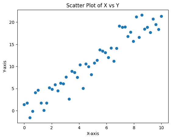
lets take 50 random points and implement gradient descent-:

we can see vizualization of data below:

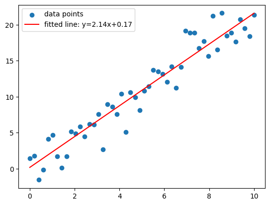
Let’s perform 100 iterations and see values of loss function and parameters at every 10th iteration.:

Iteration 0:  Loss=158.2773, m=1.4396, c=0.2184
Iteration 10: Loss=4.2799,  m=2.0871, c=0.3446
Iteration 20: Loss=4.2722,  m=2.0830, c=0.3719
Iteration 30: Loss=4.2653,  m=2.0791, c=0.3978
Iteration 40: Loss=4.2590,  m=2.0754, c=0.4225
Iteration 50: Loss=4.2533,  m=2.0719, c=0.4460
Iteration 60: Loss=4.2482,  m=2.0686, c=0.4683
Iteration 70: Loss=4.2436,  m=2.0654, c=0.4895
Iteration 80: Loss=4.2394,  m=2.0624, c=0.5096
Iteration 90: Loss=4.2356,  m=2.0595, c=0.5288

we can see the final values of parameters and loss function below:

full python code -: github

Stochastic Gradient Descent (SGD)

The problem with vanilla gradient descent is it considers all data points for updating parameters in each epoch, instead of this SGD selects one random points and updates parameters for minimizing loss function. SGD is very good for large data sets for smaller data sets SGD may not be that good.

code for SGD vs Vanilla gradient descent :- github

Momentum

This is inspired from physics where we add some percentage of velocity from previous iteration. Momentum helps the optimizer to navigate through ravines (areas where the surface curves much more steeply in one dimension than in another) more efficiently.

The formula for Momentum is:

v_t = β * v_{t-1} + (1 - β) * ∇J(θ_t)
θ_{t+1} = θ_t - α * v_t

Where:

• v_t is the velocity vector at time step t
• β is the momentum coefficient (typically 0.9)
• ∇J(θ_t) is the gradient of the cost function with respect to parameters θ at time step t
• α is the learning rate
• θ_t represents the parameters at time step t

RMSprop

In vanilla gradient descent the learning rate is fixed, which may cause oscillation in gradient descent. RMSprop (Root Mean Square Propagation) addresses this issue by adapting the learning rate for each parameter based on the history of gradients for that parameter.

RMSprop keeps a moving average of the squared gradients for each parameter and then divides the learning rate by the square root of this average. This adaptive approach allows larger updates for infrequent parameters and smaller updates for frequent parameters, which helps in faster convergence and avoiding oscillations.

The formula for RMSprop is:

E[g^2]_t = β * E[g^2]_{t-1} + (1 - β) * (∇J(θ_t))^2
θ_{t+1} = θ_t - α * ∇J(θ_t) / (√E[g^2]_t + ε)

Where:

• E[g^2]_t is the exponentially decaying average of squared gradients at time t
• β is the decay rate (typically 0.9)
• ∇J(θ_t) is the gradient of the cost function
• α is the learning rate
• ε is a small constant added for numerical stability)(avoids deviding by zero)
• θ_t represents the parameters at time step t

Adam

Adam (Adaptive Moment Estimation) combines the benefits of both Momentum and RMSprop by keeping track of two moving averages:

1.) Mean of gradients (first moment) - similar to Momentum

2.) Variance of gradients (second moment) - similar to RMSprop

Adam adapts the learning rate for each parameter by leveraging both the average of gradients (direction) and the average of squared gradients (magnitude). This makes it particularly effective for problems with noisy or sparse gradients and non-stationary objectives.

The algorithm also includes bias correction for the estimates of the first and second moments, which helps in the initial phase of training when the moving averages are biased towards zero.

Steps in Adam algorithm:

1. Initialize parameters:
   • Initialize parameters θ
   • Initialize first moment vector m₀ = 0
   • Initialize second moment vector v₀ = 0
   • Initialize timestep t = 0
2. Update parameters (for each iteration):
   • t = t + 1
   • Compute gradient g_t = ∇J(θ_t)
   • Update biased first moment estimate: m_t = β₁ * m_{t-1} + (1 - β₁) * g_t
   • Update biased second moment estimate: v_t = β₂ * v_{t-1} + (1 - β₂) * g_t²
   • Compute bias-corrected first moment estimate: m̂_t = m_t / (1 - β₁ᵗ)
   • Compute bias-corrected second moment estimate: v̂_t = v_t / (1 - β₂ᵗ)
   • Update parameters: θ_t = θ_{t-1} - α * m̂_t / (√v̂_t + ε)

The complete formula for Adam is:

m_t = β₁ * m_{t-1} + (1 - β₁) * g_t
v_t = β₂ * v_{t-1} + (1 - β₂) * g_t²
m̂_t = m_t / (1 - β₁ᵗ)
v̂_t = v_t / (1 - β₂ᵗ)
θ_{t+1} = θ_t - α * m̂_t / (√v̂_t + ε)

Where:

• m_t is the first moment estimate (mean) at time t
• v_t is the second moment estimate (variance) at time t
• m̂_t and v̂_t are the bias-corrected estimates
• β₁ and β₂ are the exponential decay rates (typically β₁ = 0.9 and β₂ = 0.999)
• g_t is the gradient at time t
• α is the learning rate
• ε is a small constant for numerical stability
• t is the timestep

Adam is currently one of the most popular optimization algorithms in deep learning because it generally outperforms other adaptive optimization methods and requires little parameter tuning.